
Overview
This project implements a full nonlinear inverted pendulum-on-cart simulator comparing two advanced control strategies: Linear Quadratic Regulator (LQR) and Model Predictive Control (MPC). The inverted pendulum is a canonical benchmark problem in nonlinear control and serves as a foundational testbed for optimization-based control methods.
The simulator models the full nonlinear dynamics of the pendulum and cart system and evaluates controller performance under different initial conditions, disturbances, weight tuning, and prediction horizons. LQR is derived from linearization and Riccati equation solutions, while MPC solves a constrained optimization problem at every timestep. The project demonstrates the difference between linear optimal control and optimization-based nonlinear control — directly reflecting advanced nonlinear and predictive control methods.
Dashboard
The Streamlit dashboard provides an interactive control simulation environment with side-panel configuration and live plots.
Initial Conditions
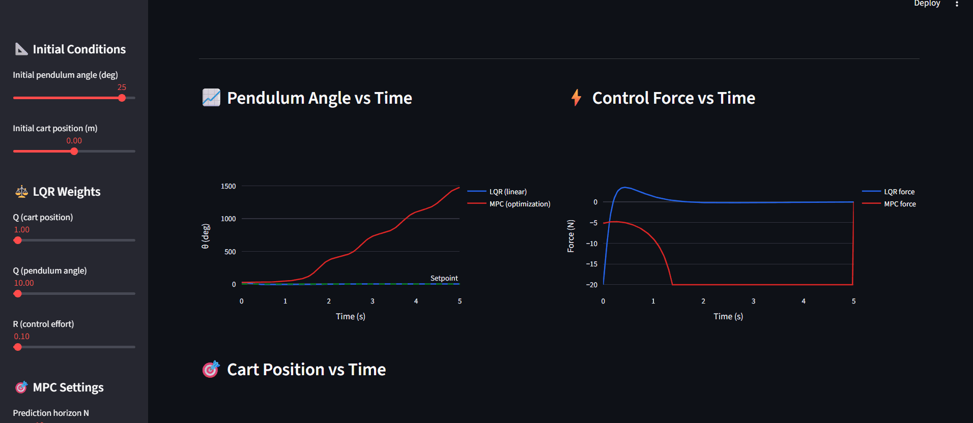
Initial pendulum angle (degrees)
Initial cart position (meters)
LQR Controller Settings
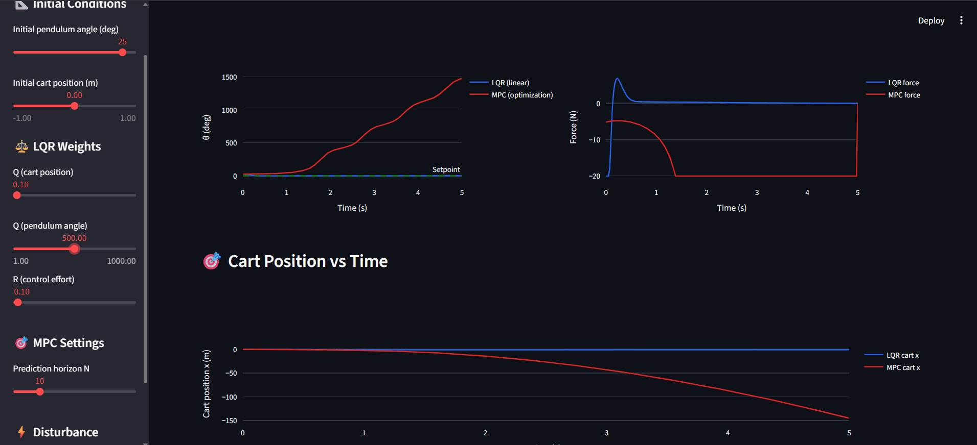
Q weight for cart position
Q weight for pendulum angle
R weight for control effort
MPC Controller Settings
Adjustable prediction horizon (N)
Disturbance Injection
Toggle disturbance
Disturbance time
Disturbance magnitude
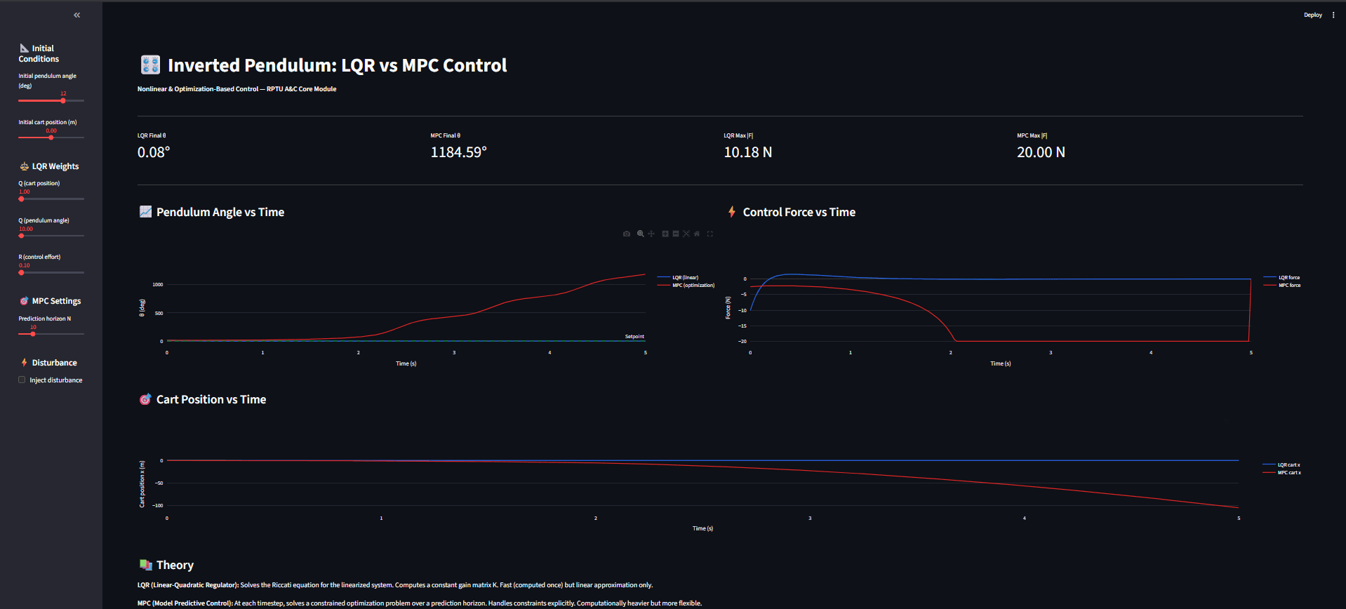
Live Outputs
KPI Cards
LQR final pendulum angle
MPC final pendulum angle
LQR maximum force
MPC maximum force
Plots
Pendulum angle vs time (LQR vs MPC)
Control force vs time
Cart position vs time
Key Engineering Concepts
Nonlinear Pendulum Dynamics
State vector:
x=[x,x˙,θ,θ˙]x=[x,x˙,θ,θ˙]
Full nonlinear equations derived from Euler–Lagrange formulation for a pendulum mounted on a moving cart.
System Linearization
Linearization around upright equilibrium enables LQR design.
State-space model:
x˙=Ax+Bux˙=Ax+Bu
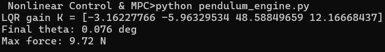
LQR (Linear Quadratic Regulator)
Solves continuous-time algebraic Riccati equation
Optimal constant feedback gain
Quadratic cost:
J=∫(xTQx+uTRu) dtJ=∫(xTQx+uTRu)dt
Fast and efficient, but based on linear approximation.
Model Predictive Control (MPC)
Solves constrained optimization over prediction horizon N
Minimizes:
J=∑k=0NxkTQxk+ukTRukJ=k=0∑NxkTQxk+ukTRuk
Handles input constraints explicitly
Re-optimizes at every timestep
More computationally expensive but robust for nonlinear regimes.
Example Scenarios / Validation
1. Large Initial Angle (Nonlinear Regime)
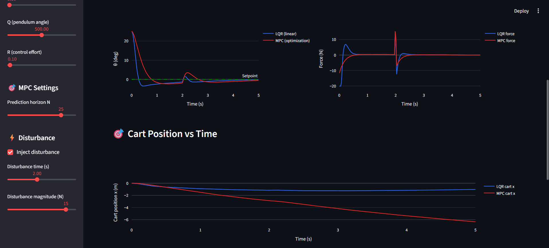
When the initial pendulum angle is increased to 25°, LQR performance degrades due to linearization assumptions, while MPC maintains better stabilization.
2. Heavy Q Weight on Angle
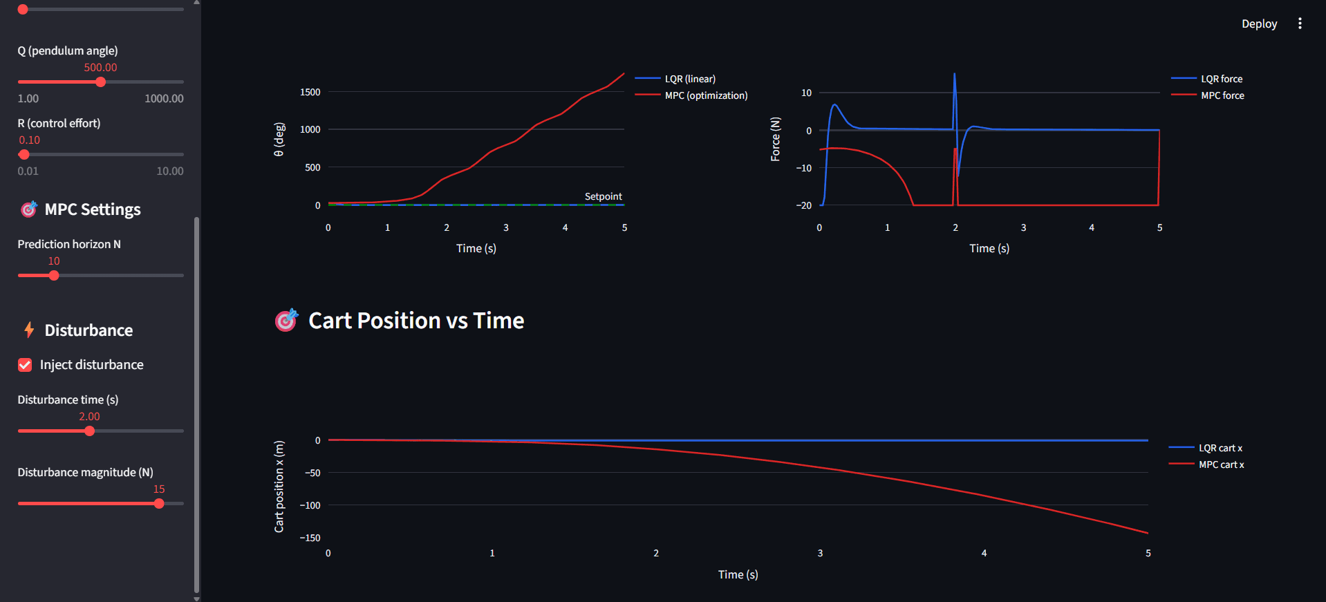
Increasing Q(θ) to 500 makes LQR more aggressive in angle correction but increases cart oscillation. Demonstrates control trade-offs.
3. Disturbance Rejection
Injecting a 15 N disturbance at t = 2 s produces a sharp deviation. MPC recovers faster due to predictive optimization.
4. Prediction Horizon Effect
Increasing MPC horizon from 10 to 25 produces smoother control trajectories but increases computation time — illustrating foresight vs complexity trade-off.
Live Demo
Open Simulator
Note: If the screen says "This app has gone to sleep due to inactivity." please click on restart app.