
Overview
Interactive A* pathfinding algorithm for autonomous robot navigation on configurable grid worlds Unmanned Systems concept
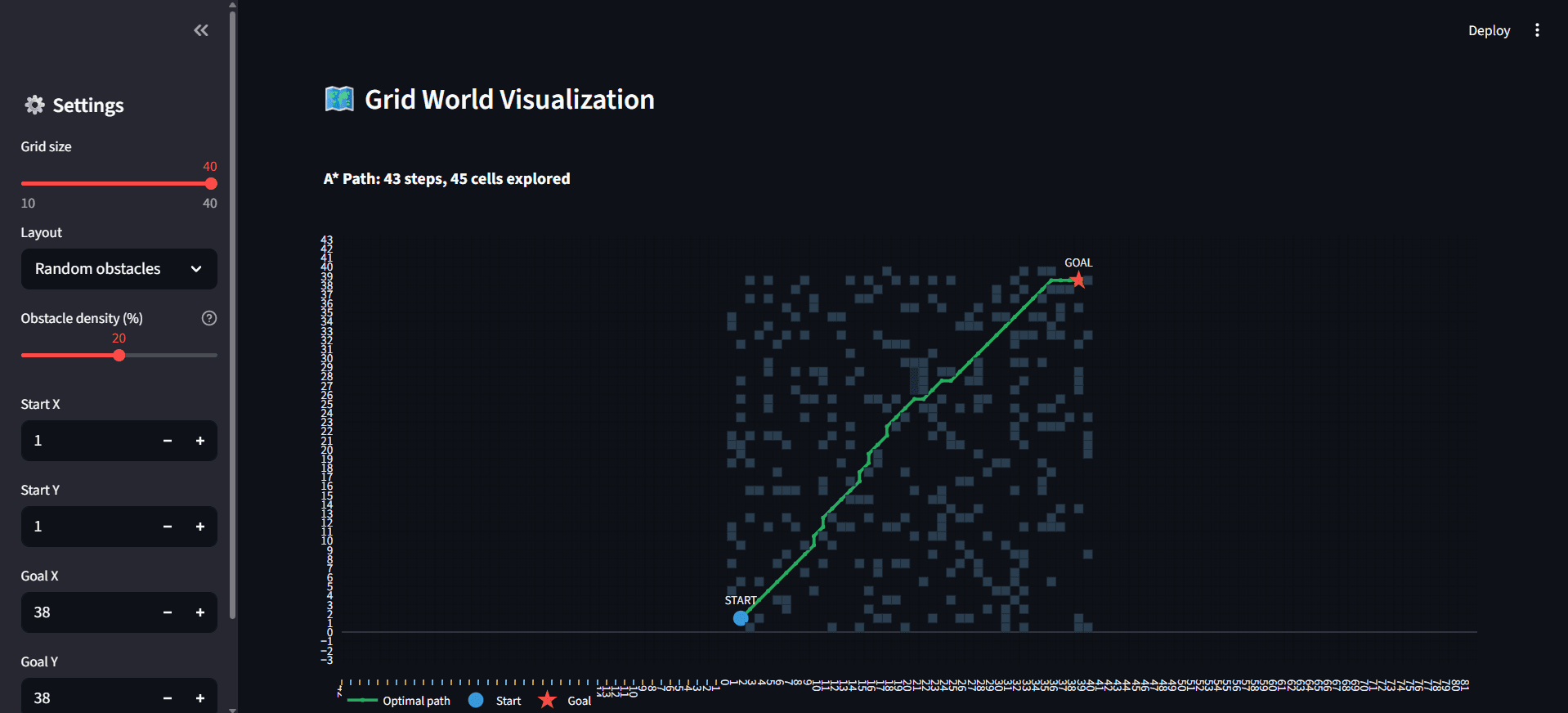
A pathfinding on a 40×40 grid with random obstacles — 43 steps, 45 cells explored
This project implements the A* pathfinding algorithm — the foundation of all autonomous robot navigation — in an interactive web simulator. A robot must find the shortest obstacle-free path from a start position to a goal position on a 2D grid world, just as a warehouse AGV, delivery robot, or unmanned aerial vehicle would in real-world autonomous operation.
The simulator supports three environment types: a structured warehouse with shelf rows and aisles, a randomly generated obstacle field with adjustable density, and an empty grid for baseline testing. Users can change the grid size (10×10 to 40×40), reposition start and goal coordinates, and watch the algorithm recompute the optimal path in real time.
Key Numbers
20×20 to 40×40 | Configurable grid worlds |
8 Directions | Cardinal + diagonal movement |
43 Steps | Optimal path through 20% obstacle density |
45 Cells | Search space explored by A* |
96% | Algorithm efficiency (path/explored ratio) |
3 Layouts | Warehouse, Random, Empty |
Pathfinding Through Obstacles
The A* algorithm combines the actual distance travelled (g-cost) with an estimated distance to the goal (h-cost, using Manhattan distance heuristic) to intelligently prioritise which cells to explore next. Unlike brute-force search algorithms that check every cell, A* focuses its exploration toward the goal — resulting in a near-optimal path while visiting far fewer cells than the total grid.
The robot moves in 8 directions: the 4 cardinal directions (up, down, left, right) at a cost of 1.0 per step, plus 4 diagonal directions at a cost of √2 ≈ 1.414 per step. This realistic cost model ensures diagonal shortcuts are used when beneficial but not over-valued.
In the visualisation, dark cells represent obstacles, the green line traces the optimal path from START (blue circle) to GOAL (red star), and light blue shading shows the search space — cells the algorithm evaluated before finding the solution. The tighter this blue region hugs the path, the more efficient the search.
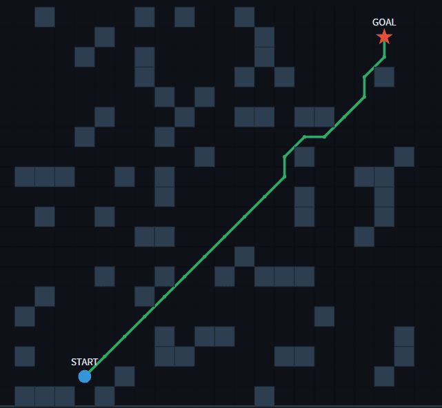
A optimal path navigating through randomly placed obstacles — the algorithm finds the shortest route while avoiding all blocked cells
Three Configurable Environments
🏭 WAREHOUSE LAYOUT Simulates a real warehouse floor with parallel shelf rows and perpendicular aisles. Shelves are placed at regular intervals with gaps every 5 cells for aisle access. The robot must navigate through these structured corridors — the same challenge faced by warehouse AGVs (Automated Guided Vehicles) in logistics centres.
🎲 RANDOM OBSTACLES Generates scattered obstacles at user-defined density (0–40%). Tests the algorithm's ability to navigate unpredictable environments — similar to outdoor terrain or cluttered workspaces where obstacle positions are not known in advance.
⬜ EMPTY GRID No obstacles — the robot takes a direct diagonal path. Serves as a baseline to verify the algorithm produces the mathematically shortest route when unobstructed (a straight diagonal line).
Performance Metrics
The dashboard calculates and displays real-time metrics for every path computation:
PATH LENGTH | Number of steps from start to goal. On a 20×20 warehouse grid, typical paths are 30–50 steps as the robot navigates around shelf rows. |
CELLS EXPLORED | Total cells evaluated by A* during search. A* explores far fewer cells than the total grid — on a 400-cell grid, it typically explores only 100–200, demonstrating the heuristic's efficiency. |
EFFICIENCY | Ratio of path length to cells explored (%). Higher efficiency means the algorithm wasted fewer evaluations. Values above 50% indicate strong heuristic guidance. |
PATH COST | Weighted distance in grid units. Straight moves cost 1.0, diagonals cost 1.414 (√2). This realistic cost model prevents the algorithm from favouring diagonals when a straight move is shorter. |
MOVE BREAKDOWN | Count of diagonal vs. straight moves — shows how the algorithm balances direct diagonal shortcuts with corridor-following straight moves. |
Features
✓ A* pathfinding algorithm with 8-directional movement (4 cardinal + 4 diagonal)
✓ Manhattan distance heuristic for optimal search guidance
✓ Realistic movement costs — straight moves: 1.0, diagonal moves: √2 ≈ 1.414
✓ Three environment types — Warehouse (structured shelves), Random (adjustable density 0–40%), Empty (baseline)
✓ Configurable grid size from 10×10 to 40×40 (up to 1,600 cells)
✓ Adjustable start and goal coordinates via sidebar
✓ Real-time path recomputation when any parameter changes
✓ Search space visualisation — explored cells shown in light blue to reveal the algorithm's decision process
✓ KPI dashboard — grid size, path length, cells explored, efficiency percentage
✓ Path detail breakdown — total cost, diagonal vs. straight move counts
✓ Deployed live on Streamlit Community Cloud
Live Demo
Note: If the screen says "This app has gone to sleep due to inactivity." please click on restart app.